A Short Reporting Window Can Understate a Campaign’s Return
A case study reports a strong return on ad spend, and the window is exactly the campaign’s live dates: launch day to the last day, nothing outside. You wonder whether the real effect was bigger than the headline, because people who saw the ads in week four cannot have bought before the report closed. That worry is fair, and it points in the opposite direction to most of what you will read about reporting windows.
The window that closes with the campaign
Most criticism of windows is about ones stretched or picked to flatter a result. This post is about a window that is short for a legitimate, defensible reason, matching the live dates, and can still mislead by understating. If you want the overclaiming side, a window picked to flatter the result covers it.
ROAS is revenue attributed to the spend divided by the spend. The spend is fixed once the campaign ends. The revenue is the part a window can shrink, because it only counts what was booked before the window shut.
Matching the window to the live dates feels rigorous for good reasons. Cost and revenue cover the same stretch of time, nobody can be accused of fishing for a flattering end date, and it is often the only clean cut available. It is a reasonable default for a case study to report. The trouble starts only when a reader takes it as the whole effect.
What carryover is, in plain terms
Someone sees the campaign, does not buy that week, and buys later because your brand is the one they remember. That is the carryover effect: exposure builds recall or consideration, and some of the purchases it produces arrive after the exposure, sometimes after the campaign has stopped. How long the lag lasts depends on the product, the price and the purchase cycle. No universal number applies, and this post will not offer one.
Marketing measurement calls this adstock, or advertising carry-over. Wikipedia’s article on advertising adstock describes it as the prolonged or lagged effect of advertising on consumer purchase behaviour, and as a model of how response builds and decays. Its companion article on marketing mix modeling says those models can account for ad stock and carry-over effects, which is one reason the technique exists. Treat both as a starting reference, not a rulebook.
Carryover is not the same thing as an attribution window. An attribution window is about how long after a click or view a conversion is still credited to it, and the attribution window is a choice, and it is rarely disclosed. Carryover is effect that persists with no tracked touch at all. A person can remember an ad, search for the brand a fortnight later, and appear in no tracked path.
A hypothetical: the same campaign, two windows
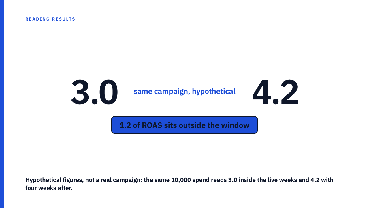
Everything in this section is hypothetical. The numbers are illustrative, not a reported result, and not a benchmark. Picture a four week campaign with 10,000 in spend. During the four live weeks, 30,000 in revenue is attributed to it. In the four weeks after it ended, a further 12,000 in revenue comes from customers who had been exposed.
| Window (hypothetical) | Spend | Attributed revenue | ROAS |
|---|---|---|---|
| Live four weeks only | 10,000 | 30,000 | 30,000 / 10,000 = 3.0 |
| Live weeks plus four weeks after | 10,000 | 30,000 + 12,000 = 42,000 | 42,000 / 10,000 = 4.2 |
| Difference | 0 | 12,000 | 1.2 |
Table caption: hypothetical figures for illustration only. They are not a real campaign and not typical of anything.
The extra 12,000 is not automatically caused by the campaign. Some of those customers would have bought anyway. So the honest reading is that the 3.0 is probably a floor on the campaign’s gross effect, not that 4.2 is the truth. The baseline question never goes away, and the counterfactual post explains why.
Why the fair reading is a floor, not a correction
A short window gives you a lower bound with an unknown gap. It does not give you licence to multiply the reported ROAS by some assumed carryover factor. That factor is unknown, and an invented multiplier is the same sin as a flattering window, committed in the other direction.
What you can do is reason about the product. A low-cost impulse purchase probably closes its gap quickly, because there is little to deliberate over. A considered purchase, something expensive or something people research and compare, can plausibly take much longer. That is reasoning about purchase cycles, not a measured fact, and it only tells you which way to lean your doubt.
Carryover also cuts against the agency in a subtler way. The weeks before a campaign can carry the effect of earlier activity, so a baseline taken right before launch can be inflated by prior spend. The live-window figure may then be understated on one side and flattered on the other. The baseline post covers how a comparison period gets chosen.
Questions to ask of the window
- Does the case study say the window ends when the campaign does? A good answer states the start and end dates of both the spend and the revenue count. If it is not stated, assume nothing about what came after.
- Is there any data after the end date? Even a single line about the following weeks helps. A good answer shows the post-campaign period alongside the live one, with the same counting rules.
- What is the typical time from first exposure to purchase for this product, and does the case study say? A good answer comes from the brand’s own sales data, not from a general claim.
- Was spend continued or replaced by other activity after the end? If so, any extended reading is muddied, because you cannot separate this campaign’s tail from the next campaign’s start.
When the case study is silent on all four, the conclusion is modest. The number is real as far as it goes, and its true size is undetermined.
Run the mirror-image test too. If a case study extends its window past the live dates, check whether it also extends the cost side, and whether the extension sweeps in seasonal or unrelated demand. A longer revenue window against a spend figure that stopped counting is a flattering mismatch, and a seasonal tailwind mistaken for campaign effect is an easy way to get one by accident.
Where the ROAS number sits in the larger picture
A bigger ROAS is not a bigger profit, so keep ROAS is not profit in mind before you get excited about 4.2 over 3.0. The cleanest answer to carryover is a holdout or incrementality design that keeps measuring after the campaign ends. Holdout tests can do that, though most published case studies do not report one.
Until then, a live-window ROAS is a floor of unknown distance from the truth. That is not a charge against whoever reported it.
Browse the case study library to practise these questions on real reports, or submit your own. In the library, every number stays credited to the agency that reported it, and the library does not restate any as a benchmark.
FAQ
What is the carryover effect in advertising?
It is the effect of advertising that persists after exposure, so purchases happen after the campaign as well as during it. Modelling work calls it adstock, and its size varies by product and cannot be assumed.
Does a short reporting window always understate ROAS?
No. It tends to understate gross effect when there is a lag between exposure and purchase, but it can be accurate for fast purchases. Treat it as a floor of uncertain distance from the truth, and do not add a multiplier, because any multiplier would be an invented number. Ask for post-campaign data or a holdout result instead.
Sources
- Advertising adstock, Wikipedia, fetched 2026-09-29
- Marketing mix modeling, Wikipedia, fetched 2026-09-29